Predicted-Flow Control Barrier Functions
for Real-Time Safe Optimal Control

Department of Mechanical & Aerospace Engineering, University of Kentucky
Preprint · 2026
FlowBarrier teaser animation

The safe set \(\mathcal{C}_{\rm s}\), the backup set \(\mathcal{C}_{\rm b}\), the closed-loop trajectory \(x(t)\), and the predicted flows \(\varphi(\tau; x, \theta, \gamma)\) along the planning time \(\tau\). At each time \(t\), the predicted flow propagates over the prediction window \([\gamma(t), T]\), remains within \(\mathcal{C}_{\rm s}\), and terminates in \(\mathcal{C}_{\rm b}\) at \(\tau = T\). The planning-time shift \(\gamma(t)\) modulates the prediction window, providing the degree of freedom that guarantees feasibility.

Abstract

Control barrier functions (CBFs) provide real-time safety guarantees through conditions on the state enforced pointwise in time. However, synthesizing a valid CBF is difficult and controllers obtained from pointwise CBF-based optimization are typically myopic. To address myopia, this article introduces predicted-flow control barrier functions (P-CBFs), which generalize the CBF concept from a function of the current state to a functional of a predicted flow under a parametrized control plan over a finite prediction horizon. For safety, a P-CBF can certify that the predicted flow is in a safe set over the entire prediction horizon. However, candidate P-CBFs suffer from the same challenge as candidate CBFs, namely, control constraints make it difficult to guarantee that the P-CBF is valid. This article resolves the validity challenge by introducing a terminal candidate P-CBF requiring that the predicted flow end in a backup safe set at the terminal time, and a planning-time shift that modulates the prediction horizon, providing an additional degree of freedom to ensure feasibility. Then, the real-time control and the evolution of the control-plan parameter and planning-time shift are determined jointly by a single convex optimization that is guaranteed to be feasible and renders the associated safe set forward invariant. The resulting safe optimal flow control provides a safety certificate over the entire prediction horizon and unifies finite-horizon integral-cost optimization with safety certification. This optimization reduces to a quadratic program (QP) if the control constraints are a convex polytope. The QP implementation, termed FlowBarrier, is validated on a nonholonomic ground robot navigating a dense environment. FlowBarrier is compared to nonlinear model predictive control and two CBF-based safety filter methods across 100 trials, where FlowBarrier achieves the highest goal-reaching rate, zero safety violations, and the lowest computation time.

1 · Preliminaries

Control Barrier Functions

Consider the control-affine system

\[ \dot x(t) = f(x(t)) + g(x(t))\,u(t), \label{eq:sys} \tag{1} \]

where \(f\colon \mathbb{R}^n \to \mathbb{R}^n\) and \(g\colon \mathbb{R}^n \to \mathbb{R}^{n \times m}\) are continuously differentiable, \(x(t) \in \mathbb{R}^n\) is the state, and \(u(t) \in \mathcal{U} \subseteq \mathbb{R}^m\) is the control. Each solution to \eqref{eq:sys} is assumed to exist and be unique on \([0,\infty)\). For notational convenience, define

\[ F(x,u) \triangleq f(x) + g(x)u, \]

which is the right-hand side of \eqref{eq:sys}.

Let \(h \colon \mathbb{R}^n \to \mathbb{R}\) be continuous, and define the zero-superlevel set \(\mathcal{C} \triangleq \{ x \in \mathbb{R}^n : h(x) \geq 0 \}\), which is assumed to be nonempty and contain no isolated points.

Let \(u_{\rm fi} \colon \mathcal{C} \to \mathcal{U}\). Then, \(\mathcal{C}\) is forward invariant with respect to \eqref{eq:sys} with \(u = u_{\rm fi}\) if for all \(x_0 \in \mathcal{C}\), the solution to \eqref{eq:sys} with \(u = u_{\rm fi}\) is such that for all \(t \in [0, \infty)\), \(x(t) \in \mathcal{C}\).

Definition 1 (Control Barrier Function)

Assume \(h\) is continuously differentiable on \(\mathcal{C}\). Then, \(h\) is a control barrier function (CBF) for \eqref{eq:sys} on \(\mathcal{C}\) if there exists an extended class-\(\mathcal{K}\) function \(\alpha\) such that for all \(x \in \mathcal{C}\),

\[ \sup_{\hat u \in \mathcal{U}} \; L_f h(x) + L_g h(x)\,\hat u + \alpha\bigl(h(x)\bigr) \;\geq\; 0. \label{eq:cbf} \tag{2} \]

Definition 1 requires that \(h\) is continuously differentiable. The next definition extends the concept of CBF to functions that are directionally differentiable but not necessarily differentiable.

The directional derivative of \(h\) at \(x\) in the direction \(\nu\) is defined by

\[ D_\nu h(x) \;\triangleq\; \lim_{s \downarrow 0} \frac{h(x + s\nu) - h(x)}{s}. \tag{3} \]
Definition 2 (Directional CBF)

Assume \(h\) is locally Lipschitz and directionally differentiable on \(\mathcal{C}\). Then, \(h\) is a directional control barrier function (D-CBF) for \eqref{eq:sys} on \(\mathcal{C}\) if there exists an extended class-\(\mathcal{K}\) function \(\alpha\) such that for all \(x \in \mathcal{C}\),

\[ \sup_{\hat u \in \mathcal{U}} \; D_{F(x,\hat u)}\, h(x) + \alpha\bigl(h(x)\bigr) \;\geq\; 0. \label{eq:dcbf} \tag{4} \]

If \(h\) is continuously differentiable, then \(D_{F(x,\hat u)} h(x) = L_f h(x) + L_g h(x) \hat u\). In this case, \eqref{eq:dcbf} is equivalent to \eqref{eq:cbf}, and Definition 2 reduces to Definition 1.

The concept of D-CBF extends to address multiple barrier functions \(h_1, \ldots, h_\ell\) and the intersection of their zero-superlevel sets \(\mathcal{C}_{\rm v} \triangleq \{x : h_1(x) \geq 0, \ldots, h_\ell(x) \geq 0\}\).

Definition 3 (D-CBF \(\ell\)-tuple)

Assume \(h_1, \ldots, h_\ell\) are locally Lipschitz and directionally differentiable on \(\mathcal{C}_{\rm v}\). Then, \((h_1, \ldots, h_\ell)\) is a D-CBF \(\ell\)-tuple for \eqref{eq:sys} on \(\mathcal{C}_{\rm v}\) if there exist extended class-\(\mathcal{K}\) functions \(\alpha_1, \ldots, \alpha_\ell\) such that for all \(x \in \mathcal{C}_{\rm v}\), \(K_{\rm v}(x)\) is nonempty, where

\[ K_{\rm v}(x) \triangleq \bigl\{ \hat u \in \mathcal{U} : D_{F(x,\hat u)} h_i(x) + \alpha_i(h_i(x)) \geq 0, \;\; i = 1, \ldots, \ell \bigr\}. \]

The next result shows that if \((h_1, \ldots, h_\ell)\) is a D-CBF \(\ell\)-tuple, then any control from \(K_{\rm v}(x)\) makes \(\mathcal{C}_{\rm v}\) forward invariant.

Theorem 1 (D-CBF Forward Invariance)

Assume \((h_1, \ldots, h_\ell)\) is a D-CBF \(\ell\)-tuple for \eqref{eq:sys} on \(\mathcal{C}_{\rm v}\), and let \(u_{\rm fi} \colon \mathcal{C}_{\rm v} \to \mathcal{U}\) be such that for all \(x \in \mathcal{C}_{\rm v}\), \(u_{\rm fi}(x) \in K_{\rm v}(x)\). Then, \(\mathcal{C}_{\rm v}\) is forward invariant with respect to \eqref{eq:sys} with \(u = u_{\rm fi}\).

2 · Predicted-Flow CBFs

From the Current State to the Predicted Flow

Let \(T > 0\) be the planning-and-prediction horizon, and consider the control plan \(u_{\rm p}(\,\cdot\,;\theta) \colon [0, T] \to \mathbb{R}^m\), which is parametrized by \(\theta \in \mathbb{R}^d\). The control plan \(u_{\rm p}\) is continuous on \([0,T] \times \mathbb{R}^d\), and for all \(\tau \in [0,T]\), \(u_{\rm p}(\tau;\,\cdot\,)\) is continuously differentiable on \(\mathbb{R}^d\). Let \(k \colon \mathbb{R}^d \to \mathbb{R}\) be continuously differentiable, and define the admissible parameter set

\[ \Theta \triangleq \{\theta \in \mathbb{R}^d : k(\theta) \geq 0\}, \]

where for all \((\tau,\theta) \in [0,T] \times \Theta\), \(u_{\rm p}(\tau;\theta) \in \mathcal{U}\).

In order to influence the time evolution of \(\theta\), let \(\theta \colon [0, \infty) \to \mathbb{R}^d\) be the solution to

\[ \dot\theta(t) = \omega(t), \qquad \omega(t) \in \Omega \subseteq \mathbb{R}^d, \label{eq:theta} \tag{5} \]

where \(\theta(0) = \theta_0 \in \mathbb{R}^d\) and \(\omega\) is the control input to the integrator.

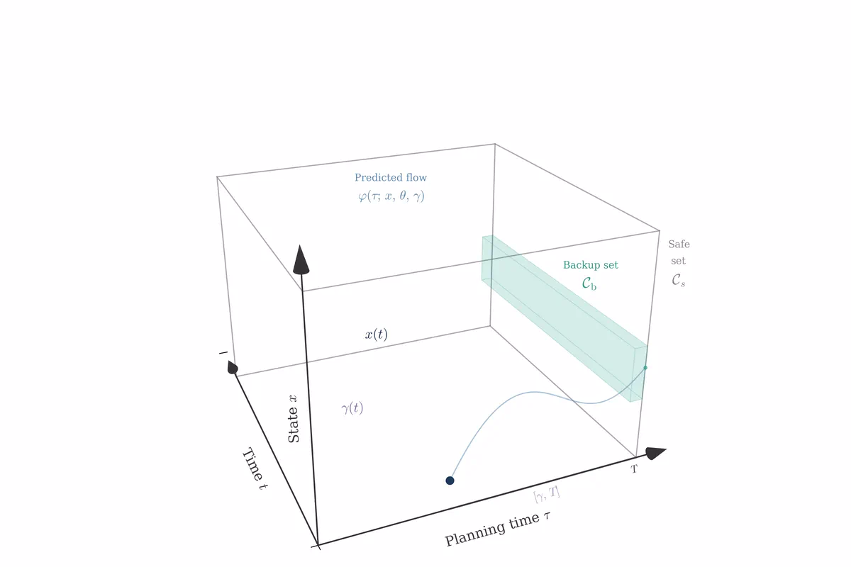
The predicted flow \(\phi(\,\cdot\,; x, \theta) \colon [0, T] \to \mathbb{R}^n\) satisfies

\[ \phi(\tau; x, \theta) = x + \int_0^\tau F\!\bigl(\phi(\sigma; x, \theta),\, u_{\rm p}(\sigma; \theta)\bigr) \, d\sigma. \label{eq:flow} \tag{6} \]

which implies that \(\phi(\tau; x, \theta)\) is the solution to \eqref{eq:sys} at planning time \(\tau \in [0,T]\) with initial condition \(x\) and \(u = u_{\rm p}(\,\cdot\,;\theta)\). In other words, \(\phi(\,\cdot\,; x, \theta)\) is the flow of \eqref{eq:sys} from state \(x\) under the plan \(u_{\rm p}(\,\cdot\,;\theta)\) with parameter \(\theta\).

Next, let \(H_1, \ldots, H_\ell \colon C([0,T], \mathbb{R}^n) \to \mathbb{R}\) be functionals such that for all \(i \in \{1, \ldots, \ell\}\),

\[ \psi_i(x, \theta) \;\triangleq\; H_i\bigl[\phi(\,\cdot\,; x, \theta)\bigr] \label{eq:psi} \tag{7} \]

is locally Lipschitz and directionally differentiable on

\[ \Psi \;\triangleq\; \bigl\{(x,\theta) \in \mathbb{R}^n \times \mathbb{R}^d : k(\theta) \geq 0,\; \psi_1(x,\theta) \geq 0, \ldots, \psi_\ell(x,\theta) \geq 0\bigr\}. \label{eq:Psi-def} \tag{8} \]

Note that \(\Psi\) is the set of \((x, \theta)\) such that the predicted flow \(\phi\) mapped through each functional \(H_i\) is nonnegative, and \(\theta \in \Theta\), which implies that \(u_{\rm p}(\tau;\theta) \in \mathcal{U}\) for the entire planning horizon \(\tau \in [0, T]\).

We now introduce the concept of a predicted-flow CBF. This concept extends the notion of a D-CBF to address the \(\ell\)-tuple \((\psi_1, \ldots, \psi_\ell)\), where each \(\psi_i\) is obtained by mapping \(\phi\) through the functional \(H_i\) and where \(k\) defines the admissible parameters for the control plan.

Definition 4 (Predicted-Flow CBF)

Assume \(\psi_1, \ldots, \psi_\ell\) given by \eqref{eq:psi} are locally Lipschitz and directionally differentiable on \(\Psi\). Then, \((\psi_1, \ldots, \psi_\ell)\) is a predicted-flow control barrier function (P-CBF) \(\ell\)-tuple for \eqref{eq:sys} and \eqref{eq:theta} on \(\Psi\) given \(u_{\rm p}\) and \(k\) if there exist extended class-\(\mathcal{K}\) functions \(\alpha_1, \ldots, \alpha_\ell, \beta\) such that for all \((x, \theta) \in \Psi\), \(K_\Psi(x, \theta)\) is nonempty, where \(K_\Psi \colon \Psi \rightrightarrows \mathcal{U} \times \Omega\) is defined by

\[ K_\Psi(x, \theta) \;\triangleq\; \bigl\{\, (\hat u, \hat\omega) \in \mathcal{U} \times \Omega \,:\, \begin{aligned}[t] &\; k'(\theta)\,\hat\omega + \beta(k(\theta)) \geq 0, \\[2pt] &\; D_{\left[\begin{smallmatrix} F(x,\hat u) \\ \hat\omega \end{smallmatrix}\right]}\, \psi_1(x, \theta) + \alpha_1(\psi_1(x,\theta)) \geq 0, \ldots, \\[2pt] &\; D_{\left[\begin{smallmatrix} F(x,\hat u) \\ \hat\omega \end{smallmatrix}\right]}\, \psi_\ell(x, \theta) + \alpha_\ell(\psi_\ell(x,\theta)) \geq 0 \,\bigr\}. \end{aligned} \]
Theorem 2 (P-CBF Forward Invariance)

Assume \((\psi_1, \ldots, \psi_\ell)\) is a P-CBF \(\ell\)-tuple for \eqref{eq:sys} and \eqref{eq:theta} on \(\Psi\), and let \(u_{\rm fi} \colon \Psi \to \mathcal{U}\) and \(\omega_{\rm fi} \colon \Psi \to \Omega\) be such that for all \((x,\theta) \in \Psi\), \((u_{\rm fi}(x,\theta), \omega_{\rm fi}(x,\theta)) \in K_\Psi(x,\theta)\). Then, \(\Psi\) is forward invariant with respect to \eqref{eq:sys} and \eqref{eq:theta} with \((u, \omega) = (u_{\rm fi}, \omega_{\rm fi})\).

3 · Problem Formulation

Safety, Cost, and Constraints

For the remainder of this article, we consider the problem of designing admissible feedback controls \((u, \omega)\) that minimize an integral cost of the predicted flow \(\phi\) over the prediction horizon such that the predicted flow \(\phi(\,\cdot\,; x(t), \theta(t))\) and actual state \(x(t)\) are in a prescribed prescribed safe set \(\mathcal{C}_{\rm s} \triangleq \{x \in \mathbb{R}^n : h_{\rm s}(x) \geq 0\}\) for all time \(t \geq 0\), where \(h_{\rm s}\) is continuously differentiable and known. We assume the admissible control sets \(\mathcal{U}\) and \(\Omega\) are convex, and \(0 \in \Omega\).

Notably, \(h_{\rm s}\) is not assumed to be a CBF for \eqref{eq:sys} on \(\mathcal{C}_{\rm s}\). Similarly, \(\psi_{\rm m}\) is not assumed to be a P-CBF for \eqref{eq:sys} and \eqref{eq:theta} on \(\Psi_{\rm m}\). Thus, it is not necessarily possible to make \(\mathcal{C}_{\rm s}\) or \(\Psi_{\rm m}\) forward invariant.

To ensure the problem is well posed, we assume there exists a subset of \(\mathcal{C}_{\rm s}\) that can be made forward invariant with respect to \eqref{eq:sys}. Specifically, consider a backup safe set \(\mathcal{C}_{\rm b} \subset \mathcal{C}_{\rm s}\), which is given by \(\mathcal{C}_{\rm b} = \{x \in \mathbb{R}^n : h_{\rm b}(x) \geq 0\}\), where \(h_{\rm b}\) is continuously differentiable and known. We make the following assumption.

Assumption 1

There exists a known extended class-\(\mathcal{K}\) function \(\alpha_{\rm b} \colon \mathbb{R} \to \mathbb{R}\) such that for all \(x \in \mathcal{C}_{\rm b}\),

\[ K_{\rm b}(x) \triangleq \{\hat u \in \mathcal{U} : L_f h_{\rm b}(x) + L_g h_{\rm b}(x) \hat u + \alpha_{\rm b}(h_{\rm b}(x)) > 0\} \]

is nonempty.

Assumption 1 implies that \(h_{\rm b}\) is a CBF for \eqref{eq:sys} on \(\mathcal{C}_{\rm b}\). Thus, \(\mathcal{C}_{\rm b}\) can be made forward invariant with respect to \eqref{eq:sys}.

Next, consider the cost \(J \colon \mathbb{R}^n \times \mathbb{R}^d \to \mathbb{R}\) given by

\[ J(x, \theta) \;\triangleq\; W\!\bigl(\phi(T; x, \theta)\bigr) + \int_{0}^{T} R\!\bigl(\phi(\tau; x, \theta),\, u_{\rm p}(\tau; \theta)\bigr)\, d\tau, \label{eq:J} \tag{9} \]

where \(W \colon \mathbb{R}^n \to \mathbb{R}\) and \(R \colon \mathbb{R}^n \times \mathbb{R}^m \to \mathbb{R}\) are continuously differentiable. The objective is formalized as follows.

Problem 1

Design feedback controls for \(u(t) \in \mathcal{U}\) and \(\omega(t) \in \Omega\) such that for each time \(t \geq 0\), the receding-horizon cost \(J(x(t), \theta(t))\) is optimized subject to the constraints:

  1. (C1) For all \((t, \tau) \in [0, \infty) \times [0, T]\), \(\phi(\tau; x(t), \theta(t)) \in \mathcal{C}_{\rm s}\).
  2. (C2) For all \(t \geq 0\), \(\theta(t) \in \Theta\).

Since \(J\) can be nonlinear and nonconvex, Problem 1 cannot necessarily be solved with a convex optimization. However, the time derivative of \(J\) along the trajectories of \eqref{eq:sys} and \eqref{eq:theta} is \(\dot J = \frac{\partial J}{\partial x}[f(x) + g(x)u] + \frac{\partial J}{\partial \theta}\omega\). To make \(\dot J\) small, consider the quadratic cost

\[ \mathcal{J}(\hat u, \hat\omega;\, x, \theta) \;\triangleq\; \tfrac{\partial J}{\partial x} g(x)\,\hat u + \tfrac{\partial J}{\partial \theta}\,\hat\omega + \hat\omega^\top Q_\omega\, \hat\omega + [\hat u - u_{\rm p}(0;\theta)]^\top Q_u\, [\hat u - u_{\rm p}(0;\theta)], \label{eq:SJ} \tag{10} \]

where \(Q_u \in \mathbb{R}^{m \times m}\) and \(Q_\omega \in \mathbb{R}^{d \times d}\) are positive definite. The first two terms make \(\dot J\) small, whereas the other two terms provide regularization that makes \eqref{eq:SJ} strictly convex. Hence, minimizing \(\mathcal{J}\) subject to (C1) and (C2) yields gradient flow that aims to decrease \(J\). Thus, we address Problem 1 by solving the following problem.

Problem 2

Design feedback controls for \(u(t) \in \mathcal{U}\) and \(\omega(t) \in \Omega\) such that for each time \(t \geq 0\), the quadratic cost \(\mathcal{J}(\hat u, \hat\omega;\, x(t), \theta(t))\) is minimized subject to (C1) and (C2).

4 · The Feasibility Gap

Solutions in Special Circumstances

The following presents solutions to Problem 2 in two special circumstances. These special circumstances can be difficult to satisfy and/or verify, which motivates the remainder of this article, where we present a solution to Problem 2 without these assumptions.

A

Solution if \(\psi_{\rm m}\) is a P-CBF

Consider the minimum-over-prediction-horizon P-CBF \(\psi_{\rm m}(x, \theta) = \min_{\tau \in [0, T]} h_{\rm s}(\phi(\tau; x, \theta))\). If \(\psi_{\rm m}\) is a P-CBF on \(\Psi_{\rm m}\), then the constraint set \(K_{\rm m}(x, \theta)\) is nonempty for all \((x, \theta) \in \Psi_{\rm m}\), and Theorem 2 implies that \(\Psi_{\rm m}\) is forward invariant.

This requires that \(\psi_{\rm m}\) is a P-CBF, which is generally difficult to satisfy and verify because it requires that for each \((x,\theta) \in \Psi_{\rm m}\), there exist \((\hat u, \hat\omega) \in \mathcal{U} \times \Omega\) satisfying the constraints in \(K_{\rm m}(x,\theta)\). In general, input constraints can lead to points where \(K_{\rm m}(x,\theta)\) is empty.

B

Solution if \((\psi_{\rm m}, \psi_{\rm t})\) is a P-CBF pair

Adding a terminal-prediction-time P-CBF \(\psi_{\rm t}(x, \theta) \triangleq h_{\rm b}(\phi(T; x, \theta))\) imposes the condition that the predicted flow terminates in \(\mathcal{C}_{\rm b}\). If \((\psi_{\rm m}, \psi_{\rm t})\) is a P-CBF pair on \(\Psi_{\rm mt} \triangleq \Psi_{\rm m} \cap \Psi_{\rm t}\), then the constraint set \(K_{\rm mt}(x, \theta)\) is nonempty for all \((x, \theta) \in \Psi_{\rm mt}\), and Theorem 2 implies that \(\Psi_{\rm mt}\) is forward invariant.

Similar to formulation A, it is generally difficult to satisfy and/or verify the condition that \((\psi_{\rm m}, \psi_{\rm t})\) is a P-CBF pair. The constraints in \(K_{\rm mt}\) are more restrictive than those in \(K_{\rm m}\), and input constraints can render \(K_{\rm mt}(x,\theta)\) empty.

5 · Planning-Time Shift

From the Feasibility Gap to Forward Invariance

This section solves Problem 2 by introducing a planning-time shift that guarantees feasibility of the optimization that determines \((u, \omega)\). The key idea is to augment the state with a planning-time shift, which allows the prediction horizon to shrink as necessary to guarantee feasibility.

Let \(\gamma \in [0, T]\) be the planning-time shift, governed by

\[ \dot\gamma(t) = z(t), \qquad z(t) \in \mathcal{Z} \subseteq \mathbb{R},\; 1 \in \mathcal{Z}. \label{eq:gamma} \tag{11} \]

Combining \eqref{eq:sys}, \eqref{eq:theta}, and \eqref{eq:gamma} yields the augmented system

\[ \dot{\bar x} \;=\; \underbrace{\begin{bmatrix} f(x) \\ 0 \\ 0 \end{bmatrix}}_{\bar f(\bar x)} \;+\; \underbrace{\begin{bmatrix} g(x) & 0 & 0 \\ 0 & I_d & 0 \\ 0 & 0 & 1 \end{bmatrix}}_{\bar g(\bar x)} \bar u, \qquad \bar x = \begin{bmatrix} x \\ \theta \\ \gamma \end{bmatrix}, \quad \bar u = \begin{bmatrix} u \\ \omega \\ z \end{bmatrix}, \label{eq:aug} \tag{12} \]

where the first block row reproduces the physical dynamics \(\dot x = f(x) + g(x) u\) of \eqref{eq:sys}, and the remaining blocks encode the integrator dynamics \(\dot\theta = \omega\) and \(\dot\gamma = z\) of \eqref{eq:theta} and \eqref{eq:gamma}. The augmented input \(\bar u = [u;\,\omega;\,z]\) lives in \(\mathcal{U} \times \Omega \times \mathcal{Z}\).

The predicted flow is extended to allow for a time shift in the control plan. The predicted flow \(\varphi(\,\cdot\,; \bar x) \colon [\gamma, T] \to \mathbb{R}^n\) satisfies

\[ \varphi(\tau; \bar x) = x + \int_\gamma^\tau F\!\bigl(\varphi(\sigma; \bar x),\, u_{\rm p}(\sigma; \theta)\bigr) \, d\sigma, \label{eq:shifted-flow} \tag{13} \]

For \(\gamma = 0\), \(\varphi\) reduces to \eqref{eq:flow}. The planning-time shift \(\gamma\) is the continuous-time analogue to shrinking the horizon in discrete-time receding-horizon control. As \(\gamma\) increases, the remaining prediction window \([\gamma, T]\) shrinks. The predicted-flow barrier functions are

\[ \bar\psi_{\rm m}(\bar x) = \min_{\tau \in [\gamma, T]} h_{\rm s}(\varphi(\tau; \bar x)), \qquad \bar\psi_{\rm t}(\bar x) = h_{\rm b}\bigl(\varphi(T; \bar x)\bigr), \label{eq:barriers} \tag{14} \]

and the associated safe set is

\[ \bar\Psi = \bigl\{ \bar x : \bar\psi_{\rm m}(\bar x) \geq 0,\; \bar\psi_{\rm t}(\bar x) \geq 0,\; k(\theta) \geq 0,\; \gamma \in [0,T] \bigr\}. \label{eq:Psi} \tag{15} \]

which is the set of \(\bar x\) such that the predicted flow satisfies \(\varphi(\tau;\bar x) \in \mathcal{C}_{\rm s}\) for all prediction times \(\tau \in [\gamma, T]\); the predicted flow satisfies the terminal condition \(\varphi(T;\bar x) \in \mathcal{C}_{\rm b}\); the control-plan parameter \(\theta\) is in the admissible set \(\Theta\); and the planning-time shift \(\gamma\) is in \([0,T]\).

Proposition 1 (Forward Invariance of \(\bar\Psi\))

Assume Assumption 1 is satisfied. Then, \(\bar\Psi\) is forward invariant with respect to \eqref{eq:aug} with \(\bar u = \bar u_{\rm fb}\), where

\[ \bar u_{\rm fb}(\bar x) = \begin{cases} [\, u_{\rm p}(\gamma; \theta);\; 0_{d};\; 1\,], & \gamma \in [0, T), \\[2pt] [\, u_{\rm b}(x);\; 0_{d};\; 0\,], & \gamma = T, \end{cases} \]

and \(u_{\rm b}\) is the minimum-norm backup controller that renders \(\mathcal{C}_{\rm b}\) forward invariant.

Proposition 1 establishes forward invariance of \(\bar\Psi\) without requiring that \((\bar\psi_{\rm m}, \bar\psi_{\rm t})\) is a P-CBF pair and without requiring pointwise nonemptiness of \(K_{\rm mt}\). The result requires only Assumption 1, which closes the feasibility gap identified in §4.

6 · Safe Optimal Flow Control

A Feasible Convex Optimization

Although \(\bar u_{\rm fb}\) makes \(\bar\Psi\) forward invariant, this control does not generally optimize the cost. Thus, this section provides a set of controls \(\bar u\) that make \(\bar\Psi\) forward invariant. Let \(\alpha_{\rm m}, \alpha_{\rm b}, \alpha_\theta, \alpha_\gamma\) be extended class-\(\mathcal{K}\) functions, and for all \(\bar x \in \{\bar x \in \bar\Psi : \gamma \neq T\}\), define the constraint set

\[ \bar K(\bar x) \;\triangleq\; \bigl\{\, \hat{\bar u} \in \mathcal{U} \times \Omega \times \mathcal{Z} \,:\, \begin{aligned}[t] &\; k'(\theta)\,\hat\omega + \alpha_\theta(k(\theta)) \geq 0, \\[2pt] &\; D_{\bar f(\bar x) + \bar g(\bar x)\hat{\bar u}}\, \bar\psi_{\rm m}(\bar x) + \alpha_{\rm m}(\bar\psi_{\rm m}(\bar x)) \geq 0, \\[2pt] &\; L_{\bar f} \bar\psi_{\rm t}(\bar x) + L_{\bar g} \bar\psi_{\rm t}(\bar x)\, \hat{\bar u} + \alpha_{\rm b}(\bar\psi_{\rm t}(\bar x)) \geq 0, \\[2pt] &\; \hat z + \alpha_\gamma(\gamma) \geq 0 \,\bigr\}. \end{aligned} \label{eq:K} \tag{16} \]
Theorem 3 (Feasibility)

For all \(\bar x \in \{\bar x \in \bar\Psi \colon \gamma \neq T\}\), \(\bar K(\bar x)\) is nonempty.

Theorem 4 (Forward Invariance)

Assume Assumption 1 is satisfied. Let \(\bar u_{\rm fi} \colon \bar\Psi \to \mathcal{U} \times \Omega \times \mathcal{Z}\) be such that for all \(\bar x \in \{\bar x \in \bar\Psi : \gamma \neq T\}\), \(\bar u_{\rm fi}(\bar x) \in \bar K(\bar x)\), and for all \(\bar x \in \{\bar x \in \bar\Psi : \gamma = T\}\), \(\bar u_{\rm fi}(\bar x) = \bar u_{\rm b}(\bar x)\). Then, \(\bar\Psi\) is forward invariant with respect to \eqref{eq:aug} with \(\bar u = \bar u_{\rm fi}\).

Consider the cost \(\bar J \colon \mathbb{R}^{\bar n} \to \mathbb{R}\) given by

\[ \bar J(\bar x) \;\triangleq\; W(\varphi(T; \bar x)) + \int_{\gamma}^{T} R(\varphi(\tau; \bar x),\, u_{\rm p}(\tau; \theta))\, d\tau, \]

which is analogous to \eqref{eq:J} except \(\phi\) is replaced by \(\varphi\). For \(\gamma = 0\), \(\bar J(\bar x)\) reduces to \(J(x,\theta)\). To make the time derivative of \(\bar J\) small, consider the quadratic cost

\[ \bar{\mathcal{J}}(\hat{\bar u}; \bar x) = w(\bar x)\, \hat{\bar u} + (\hat u - u_{\rm p}(\gamma;\theta))^\top Q_u (\hat u - u_{\rm p}(\gamma;\theta)) + \hat\omega^\top Q_\omega \hat\omega + Q_z \hat z^2 + \lambda \hat z, \label{eq:Lp} \tag{17} \]

where \(Q_u, Q_\omega \succ 0\), \(Q_z > 0\), and \(\lambda \geq 0\). The first three terms make \(\dot{\bar J}\) small, and the next three terms provide regularization that makes \eqref{eq:Lp} strictly convex. The final term \(\lambda \hat z\) penalizes increasing \(\gamma\), which incentivizes a large planning horizon \(T - \gamma\).

The safe optimal flow control is

\[ \bar u_*(\bar x) = \begin{cases} \displaystyle \operatorname*{argmin}_{\hat{\bar u} \in \bar K(\bar x)} \bar{\mathcal{J}}(\hat{\bar u}; \bar x), & \gamma < T, \\[4pt] \bar u_{\rm b}(\bar x), & \gamma = T. \end{cases} \label{eq:pi} \tag{18} \]
7 · Implementation

Quadratic Program Implementation

If \(\mathcal{U}\), \(\Omega\), and \(\mathcal{Z}\) are convex polytopes, then all constraints that define \(\bar K(\bar x)\) are affine. In this case, the safe optimal flow control \eqref{eq:pi} is the solution to the following quadratic program:

Quadratic Program \[ \bar u_{\rm p*}(\bar x) \;=\; \operatorname*{argmin}_{\hat{\bar u} \,\in\, \mathcal{U} \times \Omega \times \mathcal{Z}} \;\bar{\mathcal{J}}(\hat{\bar u};\, \bar x) \]

subject to

\[ \begin{aligned} &\; k'(\theta)\,\hat\omega + \alpha_\theta(k(\theta)) \geq 0, \\[2pt] &\; D_{\bar f(\bar x) + \bar g(\bar x)\hat{\bar u}}\, \bar\psi_{\rm m}(\bar x) + \alpha_{\rm m}(\bar\psi_{\rm m}(\bar x)) \geq 0, \quad \forall\, \tau \in \overline{\mathcal{T}}(\bar x), \\[2pt] &\; L_{\bar f} \bar\psi_{\rm t}(\bar x) + L_{\bar g} \bar\psi_{\rm t}(\bar x)\, \hat{\bar u} + \alpha_{\rm b}(\bar\psi_{\rm t}(\bar x)) \geq 0, \\[2pt] &\; \hat z + \alpha_\gamma(\gamma) \geq 0. \end{aligned} \]

This QP is guaranteed to be feasible (Theorem 3), and its solution renders \(\bar\Psi\) forward invariant (Theorem 4), which guarantees that the predicted flow and the actual state remain in \(\mathcal{C}_{\rm s}\) for all \(t \geq 0\).

Three implementation challenges arise when solving this QP in real time.

I

Semi-Infinite Program

Challenge

Since \(\overline{\mathcal{T}}(\bar x)\) may contain infinitely many points, the safety constraint may yield infinitely many affine constraints, while all other constraints are finite. Thus, the QP is a semi-infinite quadratic program.

Resolution

Replace \(\overline{\mathcal{T}}(\bar x)\) with the finite-set approximation

\[ \overline{\mathcal{T}}_{\rm e}(\bar x) \triangleq \operatorname*{argmin}_{i \in \{0,\ldots,N\}} h_{\rm s}(\varphi(\gamma + i T_{\rm s};\, \bar x)), \]

where \(T_{\rm s} = (T - \gamma)/N\). This yields a QP with finitely many affine constraints. The approximation converges to \(\overline{\mathcal{T}}\) as \(N \to \infty\).

II

Sensitivity Computation

Challenge

Solving the QP requires computing the gradients of \(\bar J\), \(\bar\psi_{\rm t}\), and \(h_{\rm s}(\varphi(\tau;\bar x))\) for all \(\tau \in \overline{\mathcal{T}}_{\rm e}(\bar x)\) with respect to \(\bar x\). The forward sensitivity method requires integrating an ODE system of dimension \(n + n(n{+}d{+}1)\), which scales with the parameter dimension \(d\).

Resolution

The adjoint method computes gradients through backward integration of an \(n\)-dimensional adjoint ODE. The complete computation consists of one forward integration of the \(n\)-dimensional state ODE followed by \((2 + N_{\rm c})\) parallel backward integrations of \(n\)-dimensional adjoint ODEs, where \(N_{\rm c} = |\overline{\mathcal{T}}_{\rm e}(\bar x)|\). Since \(N_{\rm c}\) is typically small (often \(N_{\rm c} = 1\)), this yields significant savings when \(d \gg n\).

III

Soft-Minimum Construction

Challenge

The preceding sections assumed a single safety barrier function \(h_{\rm s}\) and a single parameter barrier function \(k\). The method extends to multiple constraints for each; however, for numerical efficiency, multiple constraints can be composed into a single continuously differentiable function using the soft minimum

\[ \operatorname{softmin}_\rho(z_1, \ldots, z_N) \triangleq -\tfrac{1}{\rho}\ln\!\Bigl(\sum_{i=1}^N e^{-\rho z_i}\Bigr), \]

which is continuously differentiable and satisfies \(\operatorname{softmin}_\rho(z_1, \ldots, z_N) \leq \min(z_1, \ldots, z_N)\), with equality in the limit as \(\rho \to \infty\).

Construction

Safety barrier. Let \(b_1, \ldots, b_{N_{\rm s}}\) be continuously differentiable functions whose zero-superlevel sets define the individual state constraints. Then

\[ h_{\rm s}(x) = \operatorname{softmin}_\kappa\bigl(b_1(x), \ldots, b_{N_{\rm s}}(x)\bigr), \]

and \(\mathcal{C}_{\rm s} \subseteq \{x : b_1(x) \geq 0, \ldots, b_{N_{\rm s}}(x) \geq 0\}\), with \(\mathcal{C}_{\rm s}\) approaching the intersection as \(\kappa \to \infty\). Similarly, \(h_{\rm b}\) is constructed using the soft minimum.

Parameter barrier. Since \(\mathcal{U}\) is a convex polytope \(\mathcal{U} = \{\hat u : A_u \hat u \preceq B_u\}\), and \(u_{\rm p}(\tau;\theta)\) lies in the convex hull of \(\theta_1, \ldots, \theta_p\), the parameter barrier is

\[ k(\theta) = \operatorname{softmin}_\varrho\bigl( \zeta(\theta_1), \ldots, \zeta(\theta_p)\bigr), \]

where \(\zeta(\theta_i) \triangleq \operatorname{softmin}_\varrho(B_u - A_u \theta_i)\). It follows that \(\Theta \subseteq \mathcal{U}^p\), and \(\Theta \to \mathcal{U}^p\) as \(\varrho \to \infty\).

8 · Application

Nonholonomic Ground Robot

We consider a nonholonomic unicycle with planar position \(q = [q_x,\, q_y]^\top\), speed \(v\), and heading \(\vartheta\). The state and control-affine dynamics take the form

\[ \dot x \;=\; \underbrace{\begin{bmatrix} v\cos\vartheta \\ v\sin\vartheta \\ 0 \\ 0 \end{bmatrix}}_{f(x)} \;+\; \underbrace{\begin{bmatrix} 0 & 0 \\ 0 & 0 \\ 1 & 0 \\ 0 & 1 \end{bmatrix}}_{g(x)} u, \qquad x = \begin{bmatrix} q_x \\ q_y \\ v \\ \vartheta \end{bmatrix}, \quad u = \begin{bmatrix} u_1 \\ u_2 \end{bmatrix}, \label{eq:uni} \tag{19} \]

where \(u_1\) is the linear acceleration and \(u_2\) is the angular velocity. The robot navigates a cluttered map of 46 circular obstacles and a wall under the input constraints \(|u_1| \leq 2\,\rm m/s^2\), \(|u_2| \leq 1\,\rm rad/s\) and the state constraint \(|v| \leq 2\,\rm m/s\). Online control uses a first-order-hold parametrization of \(u_{\rm p}\) with \(p = 80\) knots over a prediction horizon \(T = 4\,\rm s\) and a discretization step \(T_{\rm s} = 0.05\,\rm s\).

FlowBarrier closed-loop demo (50× playback)

Blue: executed trajectory \(x(t)\).  Cyan dashed: predicted flow \(\varphi(\tau; \bar x(t))\).  Orange dashed: zero-level set of \(h_{\rm b}\) evaluated at the predicted terminal state. Playback \(\sim 50\times\) real time; simulated horizon \(20\,\rm s\).

Monte-Carlo Comparison

We evaluate FlowBarrier against three baselines on a benchmark of 100 navigation tasks built from a 10×10 grid of initial and goal configurations. All methods share the same cost \(J\), horizon \(T = 4\,\rm s\), discretization step \(T_{\rm s} = 0.05\,\rm s\), and input bounds; only method-specific gains are tuned individually. A trial is classified as reached if \(\|x(t) - x_{\rm d}\| \leq 0.5\,\rm m\) within \(20\,\rm s\), stuck if it fails to make progress, and failed if a safety constraint is violated.

Closed-loop trajectories for FlowBarrier, NMPC, CiLQR-CBF, and CiLQR-BCBF across 100 navigation trials.

Closed-loop trajectories for FlowBarrier, NMPC, CiLQR-CBF, and CiLQR-BCBF across 100 navigation trials in a dense obstacle environment. Trajectories are color-coded by task outcome: reached, stuck, and failed. The highlighted black trajectory in the FlowBarrier panel corresponds to the navigation task shown in the animation above.

FlowBarrier reaches the goal in 88 of 100 trials with zero failures; NMPC reaches 85, CiLQR-BCBF reaches 44, and CiLQR-CBF reaches 37 while also exhibiting 8 safety failures. Beyond outcome counts, the figure below summarizes how each method achieves its result, reporting efficiency, cost, and safety margin along both the executed and the predicted trajectory.

Monte-Carlo statistics: time-to-goal, cumulative cost, per-step computation time, barrier values, and prediction violations.

Statistical comparison of performance metrics across 100 navigation trials for FlowBarrier, NMPC, CiLQR-CBF, and CiLQR-BCBF. Metrics include time to goal, cumulative cost, computation time, minimum barrier over time \(\min_{t \in [0,20]} h_{\rm s}(x(t))\), minimum barrier over prediction horizon \(\min_{t \in [0,20],\, \tau \in [0,T]} h_{\rm s}(\varphi(\tau; \bar x(t)))\), and prediction violations.

FlowBarrier achieves the lowest per-step computation time of the four methods, approximately \(7\times\) faster than NMPC, while also reaching the goal on the largest fraction of trials and recording no safety failures. CiLQR-CBF is the only method with executed-trajectory safety violations, caused by QP infeasibility under input constraints; NMPC and CiLQR-BCBF maintain \(h_{\rm s}(x) \geq 0\) on the executed trajectory. Prediction violations, which measure whether the planned trajectory itself stays safe, are absent for FlowBarrier and present to varying degrees for every other method.

Citation

BibTeX

@misc{safari2026flowbarrier,
  author        = {Safari, Amirsaeid and Hoagg, Jesse B.},
  title         = {Predicted-Flow Control Barrier Functions for Real-Time Safe Optimal Control},
  year          = {2026},
  eprint        = {2606.00297},
  archivePrefix = {arXiv},
  primaryClass  = {eess.SY}
}